Connect to a CAN Bus: Identify Parameters and Understand Messages and Signals

BMCLI connects CAN parameter verification, message acquisition, and DBC signal decoding into a complete initial analysis. Starting with the first device connection, this article shows how AI can help find useful information in scrolling bus traffic.

Imagine a supplier delivering a controller for integration, with a DBC attached, while bench wiring records and current communication parameters are still incomplete. The engineer wants an initial report confirming which messages appear normally, followed by plots of signals relevant to the operating condition.

Prepare a computer, a BUSMUST analyzer supporting the bus, a powered target node, and a matching DBC. This article links parameter checks, capture, and signal analysis; in a separate practice environment, another analyzer can transmit teaching data in place of the real node.

Input for AI: Describe the Bus Analysis Task

Provide the project DBC, device wiring and port descriptions, and the operating conditions you may observe. Device identifiers and paths below come from the teaching bench; replace them with your project values.

For a real project, describe the task in a little more detail:

I am integrating a controller. 10357/0 connects to the target CAN bus, and the project DBC is at network/vehicle-demo.dbc. Use BMCLI to confirm the port from the wiring notes and existing Bench, discover parameters passively, then capture 30 seconds in listen-only mode. Report IDs, frame counts, periods, and bus load, and decode with the DBC to summarize key signal ranges and trends. Deliver a Markdown analysis report, trend plots, and the raw capture. Confirm any uncertain connection or database-matching issues with me.

AI first confirms the channel, then uses BMCLI to gather raw frames, statistics, and DBC engineering values before preparing the report. Parameter discovery, message identification, and exporting curves become one connected task.

Finished Result: A Set of Decoded Values

The request calls for a 30-second analysis report and trend plots. The five teaching frames below illustrate the report’s decoding section; they do not mean a complete 30-second analysis has been run for this article. Record the actual sampling duration and operating conditions in your report to support comparisons between sessions.

The example network has one VehicleStatus message with four signals: Speed, Gear, Counter, and Checksum. The transmitter changes speed in engineering units, and the receiver decodes it through the DBC:

Transmission order	Raw data	Speed	Gear	Counter
1	`00 00 00 00 00 00 00 A5`	0 km/h	P	0
2	`D0 07 03 00 00 00 01 A5`	20 km/h	D	1
3	`88 13 03 00 00 00 02 A5`	50 km/h	D	2
4	`60 22 03 00 00 00 03 A5`	88 km/h	D	3
5	`E0 2E 03 00 00 00 04 A5`	120 km/h	D	4

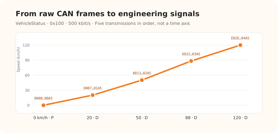
Decoded results from five VehicleStatus transmissions

Figure 2-1. Speed values from five controlled transmissions; the horizontal axis is transmission order.

All five frames were received and decoded correctly. Speed changes and gear transitions are much clearer than raw bytes. Checksum is fixed at 165 in this data to demonstrate reading a field; the node simulation example introduces checksum algorithms later.

Implementation Explained: BMCLI’s Role in the Tool

The key calls below explain the implementation. AI-generated code organizes them into a complete workflow, processes responses, and handles cleanup.

From Raw Frames to Engineering Values

The workflow uses three core command groups:

# Discover bus parameters passively without probe frames; the device must be idle and the bus must have natural traffic.
bmcli channel autoset --channel=10357/0 --mode=passive `
  --timeout=10000 --format=json

# Load the database as a named resource for later decoding or protocol operations.
bmcli database load --file=network/vehicle-demo.dbc `
  --name=tutorial-vehicle-demo --format=json
# List DBC messages to check which IDs should appear on the bus.
bmcli dbc message list --database=tutorial-vehicle-demo --format=json
# Inspect the selected message's signal layouts, scaling, and units.
bmcli dbc signal list --message=VehicleStatus `
  --database=tutorial-vehicle-demo --format=json

# Capture on the selected channel; --decode also outputs database-decoded engineering values.
bmcli message recv --channel=10357/0 --duration=30 --decode `
  --database=tutorial-vehicle-demo --format=jsonl

channel autoset discovers parameters; database load registers a named DBC resource; message recv --decode provides signal interpretation during reception. AI also organizes channel opening, listen-only configuration, and cleanup according to the bench.

BMCLI handles DBC byte order, scaling, and enumerations. For example, Speed raw 7250 becomes 72.5 km/h, and Gear 3 becomes D. AI uses these fields in reports and plots without writing another DBC parser.

Decoding preserves observed values so analysis can apply project ranges and validity rules. Encoding prepares data for transmission and checks input ranges against the DBC. Together, they support the progression from observation to controlled transmission.

For bus load and controller error counts, also use stat start/show/stop. Receive-result gaps/dropped describes data loss in the observation path, while Counter represents the application’s message count. Using both helps locate problems.

Make the Analysis More Informative

Passive discovery depends on natural bus traffic. On a quiet bench, observe longer or use project-confirmed parameters. If only Classic CAN frames appear, confirm the CAN FD data bitrate from project materials. AutoSet requires exclusive device access, so run it while the target device is idle.

Check DBC matching in stages: first IDs and lengths, then units, ranges, and responses to operating conditions. A constant signal may simply reflect a condition that has not occurred. When a value looks unreasonable, check database version, byte order, and scaling; this is easier to diagnose than changing several parameters at once.

The public DBC and bench notes are in this article’s example.

Explore Further: From Signal Curves to Troubleshooting

You can refine this example or extend it to other work. Choose a direction that interests you and discuss its implementation with AI.

A speed curve alone may not explain an anomaly. Ask AI to decode gear, brake request, and speed together, align them by receive timestamp, and mark state transitions. BMCLI reads and interprets signals; AI selects windows and organizes charts. If message periods differ, retain actual sample points and missing intervals. This gives the curve operating context and helps answer whether a change occurred before or after an action.

Check Message Timing Health

For intermittent pauses, capture longer and ask AI to calculate period distributions, maximum gaps, and anomaly times per ID, alongside bus load. For messages with counters, check increments and wrapping using the protocol’s modulus, showing application counter jumps separately from observation-path loss. Attach raw frames around anomalies for verification. The result is a report with diagnostic clues, rather than only statistics sorted by ID.