Node Simulation: Bring Virtual Nodes into Real Development and Testing

Node simulation lets a bench stand in for ECUs not yet connected and exchange messages with a real device under test. This article shows how AI and BMCLI build that communication environment, progressing from one virtual node to restbus simulation.

Imagine developing a controller that communicates with an engine ECU, power steering, airbags, and other nodes. The laboratory need not connect the whole vehicle network every time. From the communication matrix and DBC, BMCLI can supply missing nodes’ periodic messages, signal changes, and required protection fields. This is a common use of restbus simulation: retain the real DUT and simulate its other communication partners.

AI turns node roles and operating conditions into configuration; BMCLI executes transmission and fault rules. Combining periodic messages is straightforward. For network management, request/response, or state dependencies, add behavior according to project specifications rather than simply looping a few frames.

We start with one VehicleStatus node and observe its input using a second analyzer channel. This is a foundation for a multinode environment. To evaluate ECU detection, timeout, and recovery, connect the real DUT and use project-defined feedback.

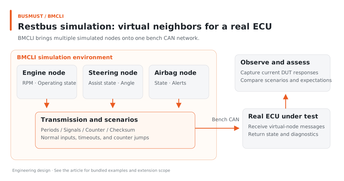
Restbus simulation: virtual neighbors for a real ECU

Figure 6-1. The bench supplies missing nodes while the ECU under test remains real. Engineering relationship diagram.

Input for AI: Describe the Node and Fault Experiments

Inputs are vehicle-demo.dbc, the demonstration counter-sum rule, and an isolated dual-channel bench. This task first verifies what the simulated node transmits; real-DUT detection and degradation testing are extensions described later.

Use BMCLI and vehicle-demo.dbc to simulate VehicleStatus with a 50 ms period. Speed varies between 40 and 80 km/h over a 2-second cycle; Gear is D. Use my demonstration counter-sum rule for Counter and Checksum. The bench is an isolated connection from 10356/0 to 10357/0. Capture 10 seconds of normal data, then run separate dropped-frame, repeated-frame, and checksum-error experiments, enabling only one fault per run and recording the rule and actual occurrence time. Deliver node configuration, raw captures, and a normal/fault comparison report, then stop this task. Use the second analyzer’s frame records as the criteria for this round.

AI writes a simulation manifest, checks it offline, and organizes each transmit/receive run. The bundled manifest already includes one message task, four signals, one waveform source, and three named faults, making it a direct starting point for changes.

Finished Result: Normal Waveforms and Fault Comparisons

Deliverables include node configuration, normal/fault captures, and a comparison report. Below are the configuration and expected frame behavior; the extensions discuss fault-tolerance testing with a real DUT.

The example sends VehicleStatus every 50 ms. Speed follows a sine wave from 40 to 80 km/h with a 2-second period, Gear stays D, and Counter/Checksum follow the demonstration rules.

After normal operation, observe three faults separately:

Scenario	Transmitter	Receiver observation
Normal node	Continuous periodic transmission	Smooth waveform and consecutive counts
Drop one frame	Do not send the selected candidate	Counter skips one value
Repeat one frame	Repeat the selected payload	Adjacent payloads repeat
Invalid checksum	Change the selected frame’s checksum field	Frame is receivable, but application checksum fails

These are the expected results for each experiment. Recording transmitter trigger counts beside received data shows whether the fault actually reached the receiver.

counter-sum here is a demonstration rule. For real projects using AUTOSAR E2E or vendor algorithms, substitute the corresponding configuration or plugin.

Implementation Explained: BMCLI’s Role in the Tool

The key calls below explain the implementation. AI-generated code organizes them into a complete workflow, processes responses, and handles cleanup.

BMCLI Manages Both Waveforms and Faults

# Check node configuration offline to confirm tasks, signals, and fault rules are understood.
bmcli simulation validate --file=vehicle-simulation.json --format=json
# Load node configuration and register the simulation name for later start and observation.
bmcli simulation load --file=vehicle-simulation.json `
  --name=tutorial-vehicle-node --format=json
# Start this simulation run and transmit continuously on the selected channel according to configuration.
bmcli simulation start tutorial-vehicle-node --channel=10356/0

# Stop this run to establish a clear boundary before changing faults or ending the experiment.
bmcli simulation stop tutorial-vehicle-node
# Enable the drop rule before restarting the task so its candidate-frame window falls within this run.
bmcli simulation fault enable drop-one --simulation=tutorial-vehicle-node
# Start this simulation run and transmit continuously on the selected channel according to configuration.
bmcli simulation start tutorial-vehicle-node --channel=10356/0
# Inspect simulation runtime state and fault trigger statistics.
bmcli simulation status tutorial-vehicle-node --format=json

# Stop this run to establish a clear boundary before changing faults or ending the experiment.
bmcli simulation stop tutorial-vehicle-node
# Disable this run's fault rule so it does not affect later experiments.
bmcli simulation fault disable drop-one --simulation=tutorial-vehicle-node

BMCLI encodes signals from the DBC and maintains periodic transmission, waveform sources, and protection fields. Values can also change by signal name at runtime:

# Update engineering values by signal name, checking and applying them as one assignment group.
bmcli simulation signal set --simulation=tutorial-vehicle-node `
  --task=vehicle --signal=Speed=65 --signal=Gear=D

The assignments are checked and applied together, avoiding partial signal updates. AI-generated scripts mainly organize experiment order, observation, and reports; periodic transmission directly reuses BMCLI.

Organize Each Experiment Run

The bundled fault window is begin=20, count=1, triggered by task candidate-frame sequence. Select the fault before starting each run so the window falls within its capture. Enabling that same window long after startup usually misses it.

stop/start restarts candidate numbering but retains signals and protection counters. To begin every run with the same initial Counter, reload this task’s configuration after stopping.

Read the current signal with bmcli simulation signal get Speed --simulation=tutorial-vehicle-node --task=vehicle. Write a name and value with --signal=Speed=42; repeat the option to update multiple signals in one call.

Also check receive-side gaps/dropped, which describes the observation path. Use Counter and checksum results to judge application faults. The host schedules simulation’s periodic tasks; combine txtask with the experiment when hardware periodic transmission is needed.

Explore Further: Give Virtual Nodes More Work

You can refine this example or extend it to other work. Choose a direction that interests you and discuss its implementation with AI.

Expand One Node into a Restbus Environment

Group missing ECUs by DBC transmitter, then supply the messages and state relationships the DUT actually depends on. This expands a single-node experiment into a restbus environment. Ask AI to use the DBC and scenario descriptions to coordinate signal changes across node configurations, with explicit periods and protection rules. BMCLI continuously transmits and changes signals; the application selects scenarios, displays stages, and records DUT responses. New scenarios become readable experiment configuration rather than another set of transmission loops.

Progress from Faulty Frames to Fault-Tolerance Tests

Suppose the specification requires an instrument to display invalid state after speed messages stop for a defined time, while counter/checksum faults follow another strategy. Observe both ends in each case:

Experiment	Input arrangement	DUT outcome to observe
Communication timeout	Stop the node for the specified interval	Does invalid state appear within the required window and clear after recovery?
Alive counter anomaly	Repeat protected frames or alter the count sequence with supported rules	Is the anomaly detected, and is stale data incorrectly accepted?
Checksum error	Keep application values reasonable and change only protection	Is invalid data rejected, and do normal frames restore processing?

Set sustained windows and expected actions from the communication specification for project tests. The three bundled frame-level experiments check injection results. After connecting the DUT, arrange sustained interruption according to timeout thresholds, then capture and assess its degradation and recovery.

Generate Fault Combinations from Communication Specifications

Timeouts, alive-counter jumps, and invalid checksums correspond to different receiver behavior. Give the specification to AI and ask for separate rules, durations, and recovery criteria for each anomaly. First check actual frames on the receive channel, then verify with the DUT. The runner enables BMCLI faults and captures feedback, while the report shows both injected inputs and receiver reactions. Retaining normal and fault scenarios separately gradually builds a regression set covering product fault tolerance.